Precision Agriculture
Remote sensing has as one of its objectives, to be able to provide useful information in the shortest possible time for decision-making. Therefore, it is considered a fundamental tool in precision agriculture, since it allows the monitoring of crops throughout the growing season, providing timely information as a diagnostic evaluation. This task must identify the factor that operates in a restrictive manner and decide, in a timely manner, on corrective agronomic intervention.
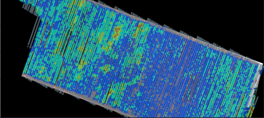
A promising approach to this is one that integrates data derived from temporal, mosaic, multispectral, and thermal imaging. Both processes allow us to obtain products such as: Thermal maps and Normalized vegetation index maps; These products allow us to identify stress zones which serve as support in agricultural management tasks.
That is why our objective is to develop an Open Source platform, distributed on a GitHub platform, that is capable of generating local calculations and mapping (plant by plant) of most important vegetation indices, through the processing of images taken with UAV.
Key words: Vegetation index, phenological status, agricultural management, Open Source platform.
Quickstart
This installation method corresponds to Debian based systems, you must find the proper libs and requirements based on your distro base that can be different.
Before You Begin: Python 3.6
If you are installing the GDAL/OGR packages into a virtual environment based on Python 3.6, you may need to install the python3.6-dev package.
sudo apt-get install python3.6-dev
Install GDAL/OGR
install the gdal-bin package (this should automatically grab any necessary dependencies, including at least the relevant libgdal version).
sudo apt-get install gdal-bin
To verify the installation, you can run ogrinfo --version.
ogrinfo --version
Install GDAL for Python
Before installing the GDAL Python libraries, you’ll need to install the GDAL development libraries.
sudo apt-get install libgdal-dev libspatialindex-dev
In order to avoid errors of missing requirement when you try to install with pip package-management system, the GDAL Python libraries version must coincide with the system installed version.
Multispectral bands
Table Nº 1: Multispectral band wavelengths available.
| Band | Wavelength |
|---|---|
| Blue | 450 nm |
| Green | 560 nm |
| Red | 650 nm |
| Red Edge | 730 nm |
| Near infrared | 840 nm |
Vegetation index calculations
The following spectral index can be generated from these lengths (Table Nº 2).
Table Nº2: Spectral index generated from the available wavelengths of camera on board UAV.
| Índex | Equation |
|---|---|
| Normalised Difference Index | NDVI = ( Rnir- Rr)/(Rnir+Rr) |
| Green Normalized Difference Vegetation Index | GNDVI = (Rnir - Rgreen)/(Rnir + Rgreen) |
| Normalised Difference Red Edge | NDRE = (Rnir - Red edge)/ (Red edge + NIR) |
| Leaf Chlorophyll Index | LCI = (Rnir - Red edge)/(Rnir + Red) |
| Optimized Soil Adjusted Vegetation Index | OSAVI = (Nir-Red)/(Nir+Red+0.16 |
Defining plant health status labels
| NDVI 1 | NDVI 1 < NDVI 2 | |
|---|---|---|
| Rank | Description | Description |
| -1 to 0 | Water, Bare Soils | Water, Bare Soils |
| 0 to 0,15 | Soils with sparse, sparse vegetation or crops in the initial stage of development (sprouting) | Poor vigor, weak plants |
| 0,15 to 0,30 | Plants in intermediate stage of development (leaf production) | Bad leaf / flower ratio |
| 0,30 to 0,45 | Plants in intermediate stage of development (leaf production) | Bad flower / fruit ratio; fruits with low sugar content, lack of color in the fruits, fruits of low caliber |
| 0,45 to 0,60 | Plants in the adult stage or phase (fruit production) | Bad flower / fruit ratio; fruits with low sugar content, lack of color in the fruits, fruits of low caliber |
| 0,60 to >0,80 | Plants in the adult stage or stage (Fruit maturity) | Bad flower / fruit ratio; fruits with low sugar content, lack of color in the fruits, fruits of low caliber |
Limitations of this solution
- The multispectral orthomosaics have to be built before using the tool.
- Charge the RGB bands separately.
- Must know the format of the bands you will be using and the metadata of each image (tiff, GeoTiff).
- In this case the methodology and support only will be for Phantom 4 RTK Multispectral user.
Methodology
To complete the main objective we consider following diagram methodology (Image Nº1). Was proposed, which reflects the process of generating the information necessary for decision- making during the management of a production cycles of a crop in general.
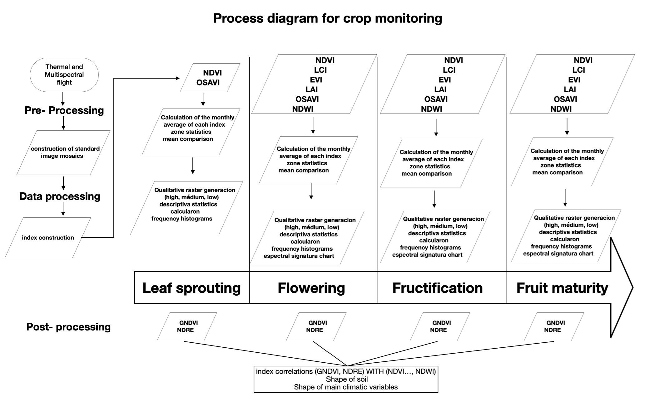
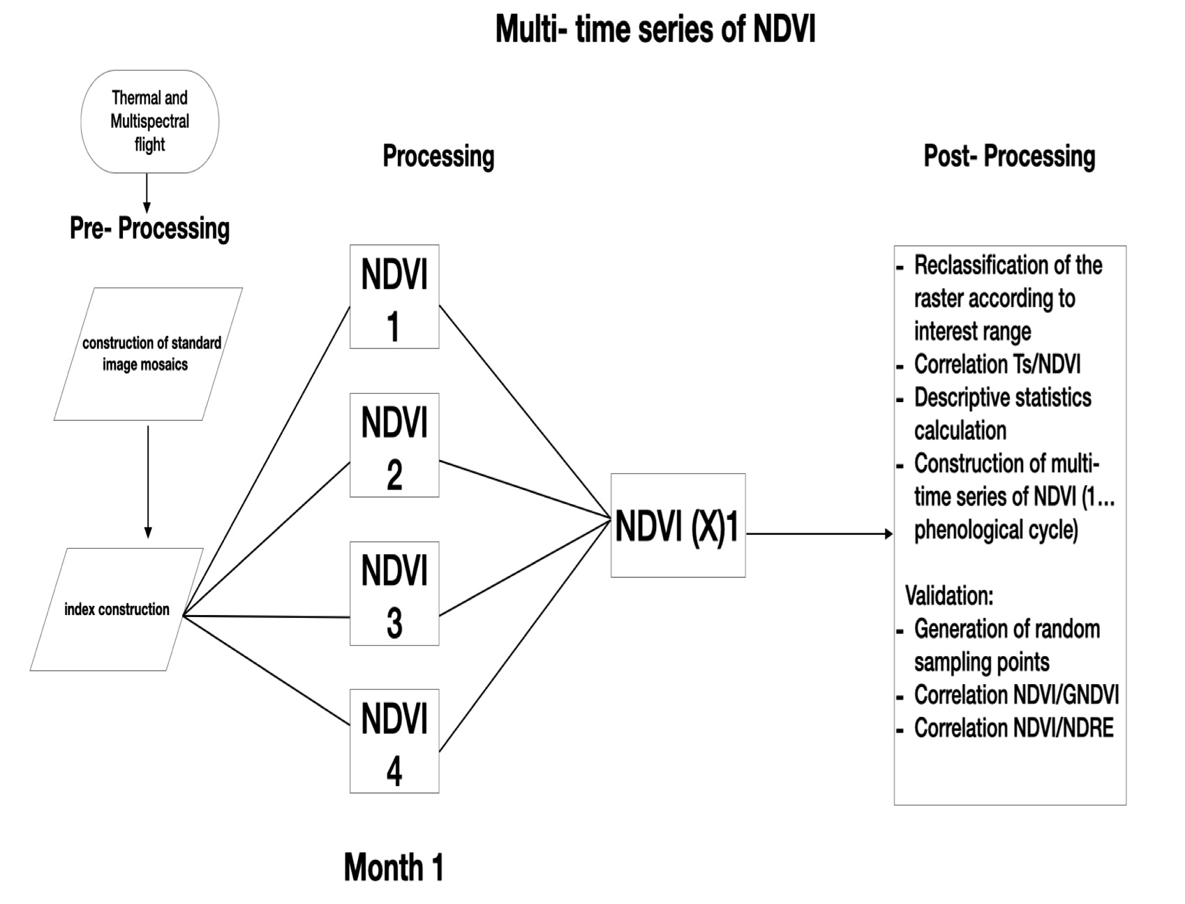
Several diagrams of sub- processes were also proposed. 1- To assess the growth status of plants. Image Nº2, NDVI multi-time series.
Data Preprocessing
Input generation to create multispectral orthomosaics
To generate the input of the Precision Agriculture algorithms of Rentadrone.cl., Which are orthomosaic of different multispectral bands, the following steps must be carried out in two well-known Open Source softwares. These are Open Drone Map and QGIS.
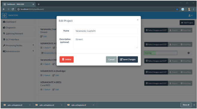
Steps in Open Drone Map (using the WebODM interface):
Add Project
Set project NAME: “Sector_Name” Description: Spectral Channel (Green)
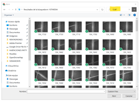
Select Images: to generate the orthomosaic of each channel (Green in this example) it is necessary to select from the dataset only of the images ending in the number corresponding to each channel image. This is number 2 for this example: DJI_0022, DJI_0032, DJI_0032. You can filter using the expression * 2.tif in the corresponding directory window.
Select Images: to generate the orthomosaic of each channel (Green in this example) it is necessary to select from the dataset only of the images ending in the number corresponding to each channel image. This is number 2 for this example: DJI_0022, DJI_0032, DJI_0032. You can filter using the expression * 2.tif in the corresponding directory window.
- For UAV DJI P4 Multispectral, he numeric endings of the files per channel are described below:
- DJI_0020.JPG (RGB)
- DJI_0021.TIFF (Blue)
- DJI_0022.TIFF (Green)
- DJI_0023.TIFF (Red)
- DJI_0024.TIFF (RedEdge)
- DJI_0025TIFF (NIR)
- For UAV DJI P4 Multispectral, he numeric endings of the files per channel are described below:
Then, we select all the filtered images and upload to our project.
- In this example we have loaded 172 images to generate the orthophoto that make up the Green channel.
In "Options" we activate
ortophoto-pngand we give it save.
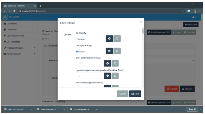
Activate
Start Processingto generate the orthophoto of the Green channel. This process must be repeated for the generation of each spectral channel.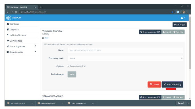
- In this example we have loaded 172 images to generate the orthophoto that make up the Green channel.
Extraction of the file already generated in this case a georeferenced orthophoto.
- After completing the process, we display the
1 Taskand download it in(GeoTiff).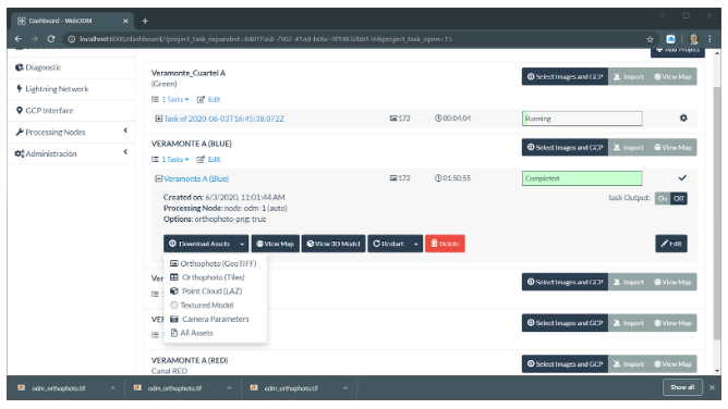 The resulting file is named
 odm_orthophoto.tiff, it only remains to rename the file in this case with the termination of the corresponding channel, in this case the image is the Blue channel.odm_orthophoto_(Project)_blue.tiffand take it to the location provided for the project.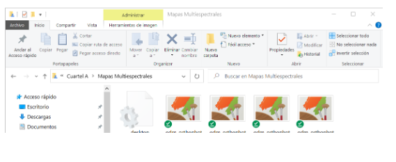
- After completing the process, we display the
Steps in QGIS:
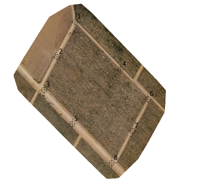
After generating the RGB orthomosaics and each of the multispectral bands: Red Edge, NIR, Red, Green, Blue, we use QGIS for their correct alignment using the Georeferencer tool, for which we have to identify distinguishable elements in both RGB orthomosaic as in each multispectral orthomosaic located on the contour of our area of interest, (example Image a) for greater precision of this process, marks or targets could be placed on the ground.
Control point distribution in RGB orthomosaic
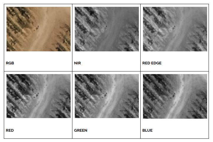
Control point for multispectral band alignment.
After identifying the control points in each image we will use QGIS to align the images using the Georeferencer tool shown below.
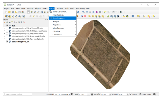
Using the Georeferencer we will be able to generate the GCPs in the RGB orthomosaic that we will use as a reference for each multispectral orthomosaic to align it to the RGB.
- step 1. open the RGB orthomosaic from the Georeferencer tool.
- step 2. identify and create the GCPs in RGB
- step 3. save the GCPs in .points format from the options window (image c)
- step 4. Open each multispectral band mosaic from the georeferencer, load the GCPs and adjust to each point separately.
- step 5. save each orthomosaic.
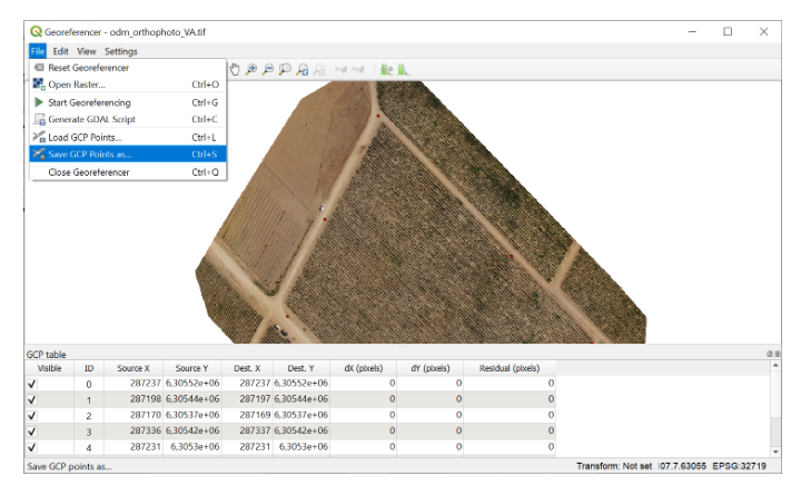
Finally, after georeferencing each Orthomosaic, the input data will be ready for the processes of calculation and mapping of vegetation indices using Rentadrone.cl's Precision Agriculture algorithms.
example of the utility
The geodata underlying the map are generate with OpenStreetMap (OSM)
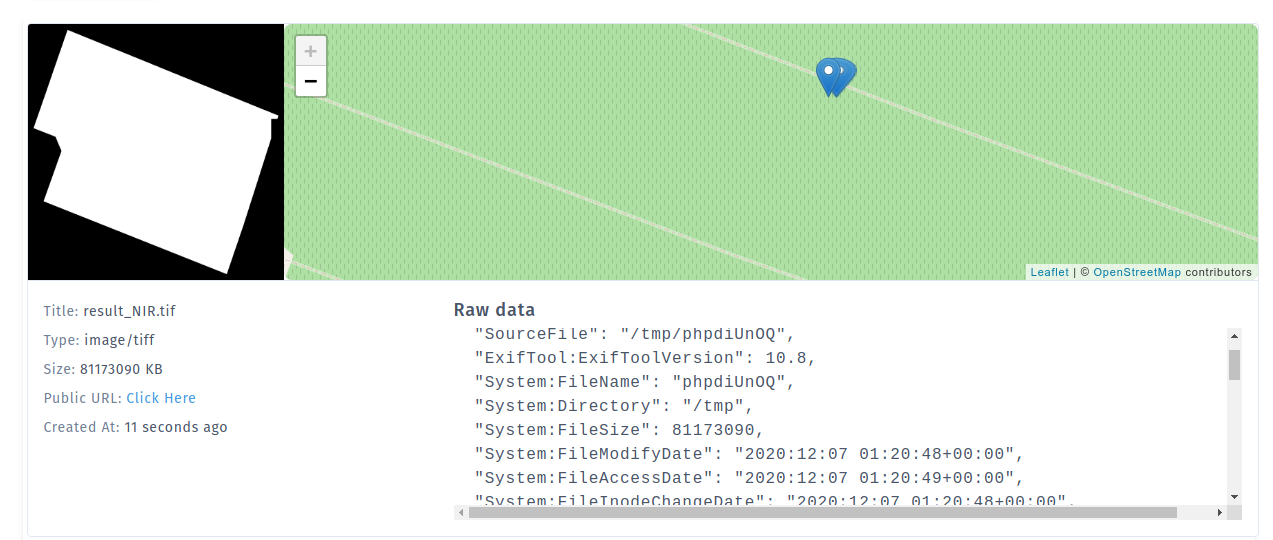
Example of an output data
GeoTIFF georeferencing information
{
  "SourceFile": "/tmp/phpdiUnOQ",
  "ExifTool:ExifToolVersion": 10.8,
  "System:FileName": "phpdiUnOQ",
  "System:Directory": "/tmp",
  "System:FileSize": 81173090,
  "System:FileModifyDate": "2020:12:07 01:20:48+00:00",
  "System:FileAccessDate": "2020:12:07 01:20:49+00:00",
  "System:FileInodeChangeDate": "2020:12:07 01:20:48+00:00",
  "System:FilePermissions": 600,
  "File:FileType": "TIFF",
  "File:FileTypeExtension": "TIF",
  "File:MIMEType": "image/tiff",
  "File:ExifByteOrder": "II",
  "IFD0:ImageWidth": 5931,
  "IFD0:ImageHeight": 5526,
  "IFD0:BitsPerSample": 32,
  "IFD0:Compression": 5,
  "IFD0:PhotometricInterpretation": 1,
  "IFD0:SamplesPerPixel": 1,
  "IFD0:PlanarConfiguration": 1,
  "IFD0:Predictor": 1,
  "IFD0:TileWidth": 256,
  "IFD0:TileLength": 256,
  "IFD0:TileOffsets": "(Binary data 4585 bytes, use -b option to extract)",
  "IFD0:TileByteCounts": "(Binary data 3237 bytes, use -b option to extract)",
  "IFD0:SampleFormat": 3,
  "IFD0:PixelScale": "5.90674417821901e-07 4.95878410333717e-07 0",
  "IFD0:ModelTiePoint": "0 0 0 -71.4437256820205 -33.3243854159711 0",
  "IFD0:GDALNoData": "nan",
  "GeoTiff:GeoTiffVersion": "1.1.0",
  "GeoTiff:GTModelType": 2,
  "GeoTiff:GTRasterType": 1,
  "GeoTiff:GeographicType": 4326,
  "GeoTiff:GeogCitation": "WGS 84",
  "GeoTiff:GeogAngularUnits": 9102,
  "GeoTiff:GeogSemiMajorAxis": 6378137,
  "GeoTiff:GeogInvFlattening": 298.257223563,
  "Composite:ImageSize": "5931x5526",
  "Composite:Megapixels": 32.774706
}
spectral index